Solving Parks (Star Battle) using Integer Optimisation
The puzzle game Parks was introduced to me by a family member who is avid player of the game. After learning the rules, it occurred to me that it might be interesting to try applying discrete optimisation techniques to solve. Parks is fairly similar to the famous eight queens puzzle, and Japanese logic puzzles like Sudoku. This blog post describes how to solve typical puzzles from the game using mixed integer linear programming (MIP).
For modelling Parks as a MIP problem, Google OR-Tools for Python was used. The non-commercial solver SCIP was used to solve the MIP problem.
I am not affiliated with the creators of Parks, however versions of the game are available to download on the Apple App Store and Google Play.
- Parks Seasons on the Apple App Store
- Parks Seasons on Google Play
Since writing the draft for this post, I found out that Parks goes by another name: Star Battle. The game was invented in 2003 by Hans Eendebak.
Introduction
Parks is a single-player logic puzzle played on a square grid of side-length \(n\). The grid is organised into \(n\) different coloured areas, called parks, where each cell in the grid belongs to one park. The goal for the player is to plant trees in cells, such that the number of trees in each row, column and park is a given number \(m\). Trees may not touch, which means that two trees may not be planted in cells that are adjacent to each other, either horizontally, vertically or diagonally.
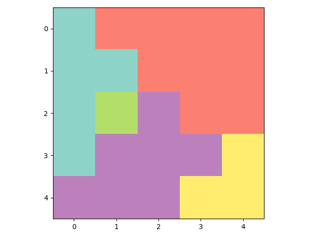
The figure below depicts an unsolved puzzle in a 5x5 grid, where one tree must be planted in each row, column and park.
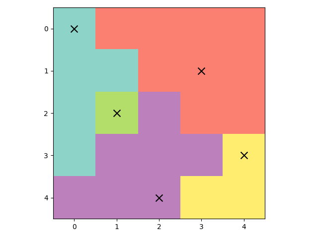
The solution to this puzzle is shown below, where trees are denoted by black crosses. You can verify that there is one tree in each row, column and park, and no two trees are planted in adjacent cells. The solution is unique.
Mathematical Model
The approach taken was to define integer decision variables to denote where trees are planted, and then to describe the rules of the puzzle in terms of linear constraints on these variables. This enables the problem to be formulated as a MIP, and given to a MIP solver such as SCIP to solve. In spite of the fact that integer programming is NP-complete, there are numerous instances of MIPs that can be solved efficiently, using methods such as branch and cut.
As a first step, let’s define the square grid of side-length \(n\) that Parks is played on as a set of grid indices \(I=\{(i,j) \vert i,j \in \{1,\dots,n\}\}\). The colour of each park is denoted by an integer from \(1\) to \(n\). The sets of grid indices belonging to each of the \(n\) parks will then form a partition \(P=\{P_{1},\dots,P_{n}\}\) of the set \(I\). Specifically, the subset \(P_{k} \in P\) contains the grid indices for the cells in park \(k\). Since \(P\) is a partition of \(I\), it holds that:
-
The set \(P\) does not contain the empty set. In other words, each park covers at least one cell, i.e. \(P_{k} \neq \emptyset\) for all \(k \in \{1,\dots,n\}\).
-
The union of the sets in \(P\) is equal to \(I\). In other words, parks cover all grid cells, i.e. \(\bigcup_{k=1}^{n} P_{k}=I\).
-
The intersection of any two sets in \(P\) is empty. In other words, parks do not overlap with each other, i.e. \(P_{k} \cap P_{l} = \emptyset\) for all \(k,l \in \{1, \dots, n\}\) where \(k \neq l\).
This definition does not mean that solving a puzzle is feasible, or that it has a unique solution, which are properties of the puzzles in the game. Also, in the game, there are a few puzzles where the parks do not cover the whole grid, meaning this definition does not apply to them. For example, some cells in the grid of a non-regular puzzle may not belong to a park, and cannot have trees planted on them.
We will model Parks as a MIP which has a solution if and only if the puzzle is feasible. Our model uses binary decision variables \(x_{ij}\) indicating whether a tree is planted in the cell with grid indices \((i,j)\), where \(x_{ij}=1\) means a tree is planted and \(x_{ij}=0\) means no tree is planted. The goal of the optimisation is to find values of the decision variables such that all the rules are respected.
The problem is then formulated by:
\[\begin{align} \sum \limits_{d_{1}=0}^{1} \sum \limits_{d_{2}=0}^{1} x_{i+d_{1},j+d_{2}} \leq 1 & \qquad \forall i,j \in \{1,\dots,n-1\} \\ \sum \limits_{j=1}^{n} x_{ij}=m & \qquad \forall i \in \{1,\dots,n\} \\ \sum \limits_{i=1}^{n} x_{ij}=m & \qquad \forall j \in \{1,\dots,n\} \\ \sum \limits_{(i,j)\in P_{k}} x_{ij}=m & \qquad \forall P_{k} \in P \\ x_{ij} \in \{0,1\} & \qquad \forall i,j \in \{1,\dots,n\} \end{align}\]The first constraint prevents trees from being planted in adjacent cells, by ensuring that each 2x2 sub-grid contains at most a single tree. This is a necessary and sufficient condition for no trees to be touching. The second constraint ensures exactly \(m\) trees are planted in each row. The third constraint ensures that exactly \(m\) trees are planted in each column. The fourth constraint ensures that exactly \(m\) trees are planted in each park. The last line in the problem formulation defines the domain of the decision variables.
The following section sets out the implementation details and some results.
Code and Results
The following Python code (GitHub repo) defines a class named ParksPuzzle. When a ParksPuzzle object is declared we pass it three parameters. These are the unsolved puzzle as an nxn array called parks, the number of required trees per park, row and column m and the side-length of the grid n. Each element of parks is an integer from 0 to n-1 to denote which park the corresponding cell belongs to. First, the code checks that the unsolved puzzle is valid. Then the class attributes that were passed in as parameters are initialised. Two more class attributes are then initialised: an nxn array for the solution called trees which is initially all zeros, and the list of grid indices corresponding to each park P.
import numpy as np
from ortools.linear_solver import pywraplp
import matplotlib.pyplot as plt


class ParksPuzzle:
    def __init__(self, parks: np.ndarray, m: int, n: int) -> None:
        """Class for a Parks puzzle game.

        Args:
            parks (np.ndarray): nxn array of park locations going from 0 to n-1
            m (int): number of trees per park, row and column
            n (int): number of parks and size of grid
        """
        parks = np.asarray(parks)

        # check that the puzzle is valid
        assert parks.shape == (n,n)
        for i in range(m):
            assert i in parks
        for i in range(n):
            for j in range(n):
                assert parks[i,j] in range(n)

        # initialise class attributes
        self.parks = parks
        self.m = m
        self.n = n

        # nxn array of tree locations
        self.trees = np.zeros((n, n))

        # element k of P is a list of grid indices for park k
        self.P = [
            [(i, j) for i in range(n) for j in range(n) if parks[i, j] == k]
            for k in range(n)
        ]
Next in the code is the method to actually solve the puzzle. I found this example, provided in the Google OR-Tools guide, to be a useful template. First the solver is instantiated. Then the (binary) decision variables are created and stored in a dictionary x where the keys are tuples of grid indices. Then each of the constraints are added to the model. The solver is called, and the solution is printed out.
    def solve(self) -> None:
        """Solve the puzzle."""
        m = self.m
        n = self.n
        P = self.P

        # Create the mip solver with the SCIP backend.
        solver = pywraplp.Solver.CreateSolver("SCIP")

        # Define the decision variables
        # x(i,j)=1 if there is a tree at grid indices (i,j)
        # otherwise x(i,j)=0
        x = {}
        for i in range(n):
            for j in range(n):
                x[i, j] = solver.BoolVar(f"x{i,j}")

        # Define the constraints
        # trees do not touch
        # i.e. each 2x2 subgrid contains no more than 1 tree
        for i in range(n - 1):
            for j in range(n - 1):
                solver.Add(
                    sum([x[i + d1, j + d2] for d1 in range(2) for d2 in range(2)]) <= 1
                )

        # m trees per row
        for i in range(n):
            solver.Add(sum([x[i, j] for j in range(n)]) == m)

        # m trees per column
        for j in range(n):
            solver.Add(sum([x[i, j] for i in range(n)]) == m)

        # m trees per park
        for k in range(n):
            solver.Add(sum([x[i, j] for (i, j) in P[k]]) == m)

        # Solve the problem
        status = solver.Solve()

        print("Number of variables =", solver.NumVariables())
        print("Number of constraints =", solver.NumConstraints())
        print()

        if status == pywraplp.Solver.OPTIMAL:
            print("Objective value =", solver.Objective().Value())
            for i in range(n):
                for j in range(n):
                    print(x[i, j].name(), " = ", x[i, j].solution_value())
            print()
            print("Problem solved in %f milliseconds" % solver.wall_time())
            print("Problem solved in %d iterations" % solver.iterations())
            print("Problem solved in %d branch-and-bound nodes" % solver.nodes())
        else:
            print("The problem does not have an optimal solution.")

        # Update trees grid
        self.trees = np.zeros((n, n))
        for i in range(n):
            for j in range(n):
                if x[i, j].solution_value() > 0.5:
                    self.trees[i, j] = 1
The final method visualises the puzzle:
    def draw(self, fname: str = None) -> None:
        """Draw parks and trees on grid.

        Args:
            fname (str, optional): Filename for saving plot. Defaults to None.
        """
        parks = self.parks
        n = self.n
        trees = self.trees

        cmap = plt.cm.Set3
        plt.figure()
        plt.imshow(parks, interpolation="nearest", cmap=cmap)

        xs, ys = np.ogrid[:n, :n]
        # the non-zero coordinates
        u = np.argwhere(trees)

        plt.scatter(
            ys[:, u[:, 1]].ravel(), xs[u[:, 0]].ravel(), marker="x", color="k", s=100
        )

        plt.tight_layout()
        if fname is not None:
            plt.savefig(fname)
        plt.show()
Simple Puzzle
Attempting to solve the 5x5 puzzle from the introduction that requires 1 tree to be planted in each row, column and park (m=1 and n=5):
puzzle = ParksPuzzle(
    parks=[
        [0, 1, 1, 1, 1],
        [0, 0, 1, 1, 1],
        [0, 2, 3, 1, 1],
        [0, 3, 3, 3, 4],
        [3, 3, 3, 4, 4],
    ],
    m=1,
    n=5,
)
puzzle.solve()
puzzle.draw()
Prints to the screen:
Number of variables = 25
Number of constraints = 31

Objective value = 0.0
x(0, 0)  =  1.0
x(0, 1)  =  0.0
x(0, 2)  =  0.0
x(0, 3)  =  0.0
x(0, 4)  =  0.0
x(1, 0)  =  0.0
x(1, 1)  =  0.0
x(1, 2)  =  0.0
x(1, 3)  =  1.0
x(1, 4)  =  0.0
x(2, 0)  =  0.0
x(2, 1)  =  1.0
x(2, 2)  =  0.0
x(2, 3)  =  0.0
x(2, 4)  =  0.0
x(3, 0)  =  0.0
x(3, 1)  =  0.0
x(3, 2)  =  0.0
x(3, 3)  =  0.0
x(3, 4)  =  1.0
x(4, 0)  =  0.0
x(4, 1)  =  0.0
x(4, 2)  =  1.0
x(4, 3)  =  0.0
x(4, 4)  =  0.0

Problem solved in 9.000000 milliseconds
Problem solved in 0 iterations
Problem solved in 0 branch-and-bound nodes
The solver found a feasible solution quite quickly in 0.009 seconds. As no objective was defined, the default value 0 is printed. This is the same solution as the one depicted earlier. For a square grid of side-length \(n\), the number of decision variables is \(n^{2}\) (the number of cells) and the number of constraints is \(n^{2}+n+1\) (the number of 2x2 sub-grids plus the number of columns, rows and parks).
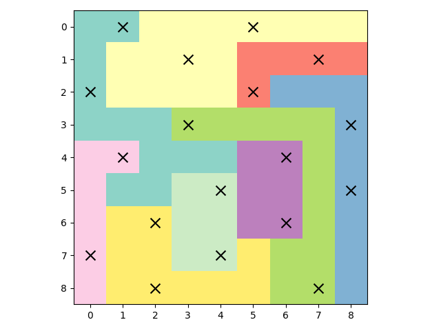
A Harder Puzzle
Now let’s solve a puzzle from later in the game. This puzzle has a 9x9 grid and requires 2 trees to be planted in every row, column and park (m=2 and n=9).
puzzle = ParksPuzzle(
    parks=[
        [0, 0, 1, 1, 1, 1, 1, 1, 1],
        [0, 1, 1, 1, 1, 2, 2, 2, 2],
        [0, 1, 1, 1, 1, 2, 3, 3, 3],
        [0, 0, 0, 4, 4, 4, 4, 4, 3],
        [5, 5, 0, 0, 0, 6, 6, 4, 3],
        [5, 0, 0, 7, 7, 6, 6, 4, 3],
        [5, 8, 8, 7, 7, 6, 6, 4, 3],
        [5, 8, 8, 7, 7, 8, 4, 4, 3],
        [5, 8, 8, 8, 8, 8, 4, 4, 3],
    ],
    m=2,
    n=9,
)
puzzle.solve()
puzzle.draw()
Prints to the screen:
Number of variables = 81
Number of constraints = 91

Problem solved in 26.000000 milliseconds
Problem solved in 36 iterations
Problem solved in 1 branch-and-bound nodes
Visualisation of the solution:
This puzzle was also solved quickly in 0.026 seconds, although it required more iterations and the branch-and-bound tree had 1 node.